RNA Model Building Workshop
1. Introduction
This workshop will give an introduction to the model building tools available in CCP4 for nucleic acid structures, using data from a published RNA structure as an example. The structure we are trying to build is 1HR2 with 2 copies of a 158-residue domain at 2.25 Å resolution (Juneau et al. 2001). The map and phases we will be starting from are from the rebuilt and re-refined model in PDB-REDO, which has an R-free value of 26.4%. This map is unrealistically good compared to one that would have be obtained after either experimental phasing or molecular replacement using a homologue or a predicted model.
Click the following files to download them to your computer:
- data.mtz - reflection data in MTZ format
- sequence.fasta - RNA sequence in FASTA format
2. CCP4i2
We will be using the CCP4i2 interface in this workshop.
It is also possible to perform the same tasks in CCP4 Cloud
but the step-by-step instructions would be slightly different.
Start CCP4i2 by double-clicking the desktop icon
(or by entering ccp4i2 on the command line)
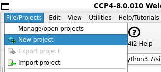
then create a new project using File/Projects / New project.
In the Create a New Project window, enter a project name
and click the Create project button.
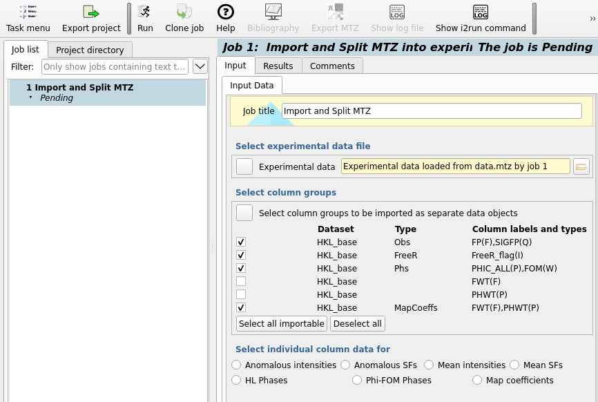
2.1. Import and Split MTZ
The first task will be to import the reflection data into CCP4i2.
Find Import and split MTZ into experimental data objects
in the task menu.
On the input tab, use the folder icon on the right
to select the data.mtz file that was downloaded earlier.
A window will open to ask about the provenance of the imported file.
If this is not something you wish to use
you can uncheck the option at the top of the window
to stop it being shown when importing a file.
Click OK to accept the default description of the source of the file.
Use the Select all importable button to select the observations (Obs),
free-R flag (FreeR), phases (Phs) and map coefficients (MapCoeffs).
Click the run button at the top of the window to finish importing the data.
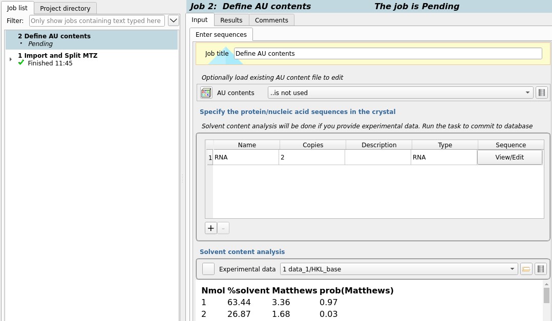
2.2. Define AU Contents
The second task to run is the Define AU contents task.
The input page allows us to specify a list of protein and nucliec acid sequences.
Use the + button on the bottom left of this box
to select the sequence.fasta file.
The sequence should be added automatically with the type of RNA.
With the sequence added, selecting Experimental data in the box below
will perform a solvent content analysis
to help guess the number of copies in the asymmetric unit (AU).
There are four entries in this dropdown -
one for each reflection data object imported,
each with the name 1 data_1/HKL_base.
However, all have the same cell and space group
so it doesn't matter which one is chosen as the volume of the AU is the same.
In this case we know there are two copies in the AU
so change the Copies field in the sequence list to 2
and run the job to create the AU contents object.
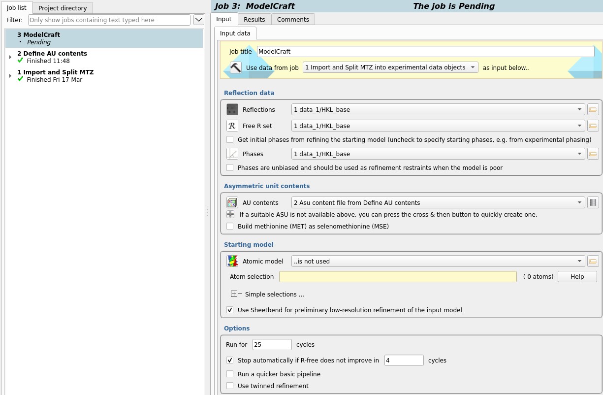
2.3. ModelCraft
Now we have the reflection data and AU contents description
we can try automated model building using ModelCraft.
This is a model building pipeline that combines
protein and nucelic acid model building using Buccaneer and Nautilus
with other programs for refinement, density modification and model validation.
Open the ModelCraft task from the task menu.
Select the Reflections and Free R set
in the Reflection data box.
As we are providing initial phases instead of getting them from a starting model,
uncheck the option at the bottom of this box
and select the Phases loaded earlier.
The phases are not unbiased (they come from the final model)
so do not check the option below.
Select the AU contents created in job 2 then run the task
with all other defaults.
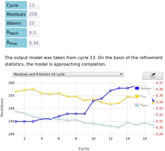
ModelCraft will take a while to run to completion, but results should start appearing in the report after the first cycle has completed. After it has finished, there should be a report similar to the following image. The pipeline has decided that the model from cycle 13 was the best model. It stopped because it did not produce a better model in cycles 14, 15, 16 or 17. ModelCraft built a model with 258 residues and a free R-factor of 34%. For comparison, the PDB-REDO model has 315 residues and a free-R factor of 24%. ModelCraft is better at building protein models than nucelic acid models. If it did not produce a good model I would recommend trying other automated model building programs such ARP/wARP (which can be accessed through CCP4 Cloud or the ARP/wARP Web Service) or PHENIX AutoBuild. While ModelCraft is running, move on to the next section to try interactive model building with Coot.
3. Coot
While ModelCraft is performing fully-automated model building,
we will introduce the interactive model building tools for nucleic acids in Coot.
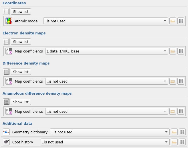
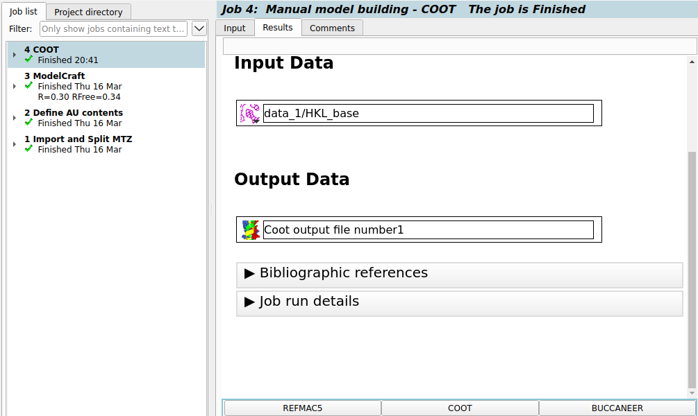
Start by finding the Manual model building - COOT task in CCP4i2.
We will just start from the map imported in job 1.
Make sure the Electron density maps selection
is set to 1 data_1/HKL_base
and all the other selections are set to ...is not used,
then run the task to open Coot.
3.1. Cootilus
Coot includes automated nucleic acid building through an adapted implementation of the Nautilus program (known as Cootilus). This implementation is faster than Nautilus because it only searches for nucleic acids within a user-specified radius of the view center. If initial residue positions are found, Cootilus will attempt to grow these into longer RNA chains. It can help to repeat this process by centering the view on parts of the RNA model that are missing or built incorrectly. This tool may overwrite and join with existing nucelic acid residues. However, it does not perform sequencing and will build all nucelic acids as uridine (U) with a truncated base.
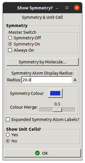
Before trying it out, turn on symmetry copies
by going to Draw / Cell & Symmetry.
Change the Master Switch to Symmetry On,
increase the Radius to 20.0 and click OK.
This will help to avoid building into symmetry copies.
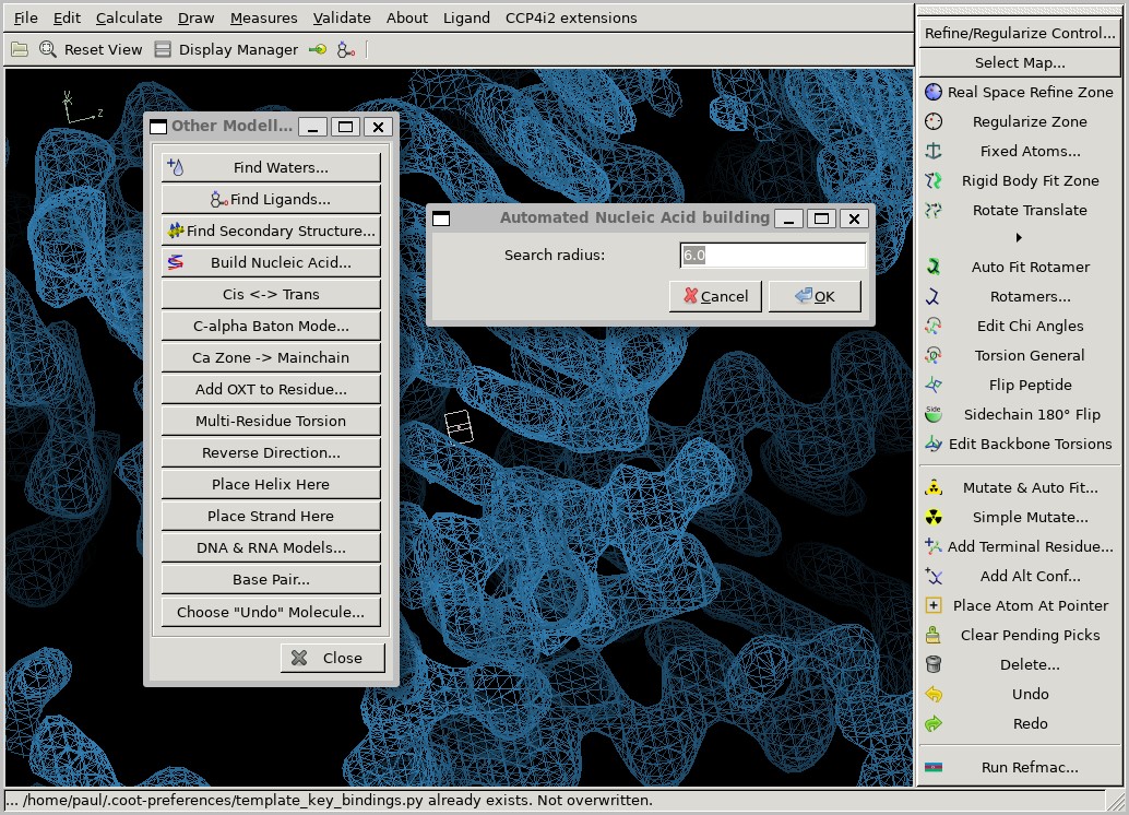
Cootilus can be found at
Calculate / Other Modelling Tools / Build Nucleic Acid.
Try to build a long single chain using this tool,
but don't spend too much time on it.
You may find it struggles to build in some areas of the map.
Increasing the Search radius parameter might help.
The Go To Atom window (shortcut F6)
will help to see the residues you have built already.
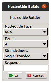
3.2. Nucleotide Builder
Also available in the Other Modelling Tools window
is the Nucleotide Builder (listed as DNA & RNA Models).
It adds a new molecule with idealised RNA or DNA
in A or B form with a specified sequence.
The Rotate / Translate tool in the refinement toolbar (on the right)
can be used to get roughly the correct position
before real-space refinement and merging into the existing molecule.
If standard real-space refinement does not work to refine the ideal strand
then it may help to try jiggle fitting instead.
To jiggle fit a single residue use the shortcut key J.
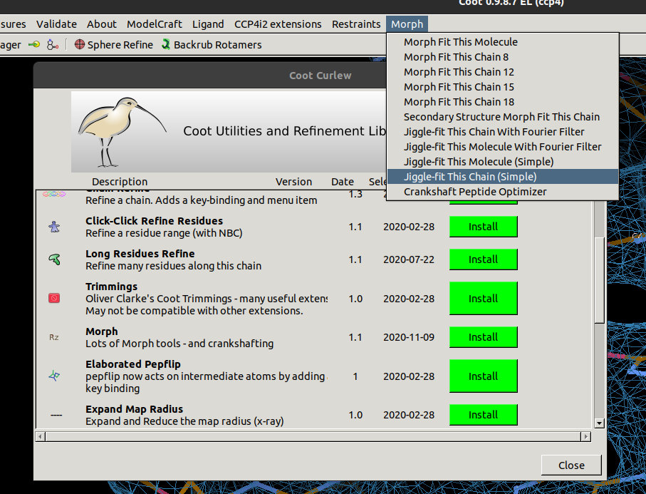
It is also possible to perform jiggle fitting on whole chains or whole molecules.
To get these options, first open
File / Curlew (the Coot extensions wrangler)
and install the Morph module.
Jiggle fitting tends to work better at lower resolution.
With higher resolution data it might help to blur the map first
from Calculate / Map Sharpening/Blurring.
3.3. Adding Residues
New adenosine residues can be added at the end of chains using the
Add Terminal Residue tool in the Refinement toolbar.
These will require some real-space refininement after they have been added.
It helps to refine the previous residue along with the new one so that
there is some flexibility in the bonding.
This can be done with the Real Space Refine Zone tool
or by using the shortcut key t (triple-refine)
to refine the residue at the center of the view and one residue either side.
If the shortcut key does not work, you may need to first click
Edit / Settings / Install Template Keybindings.
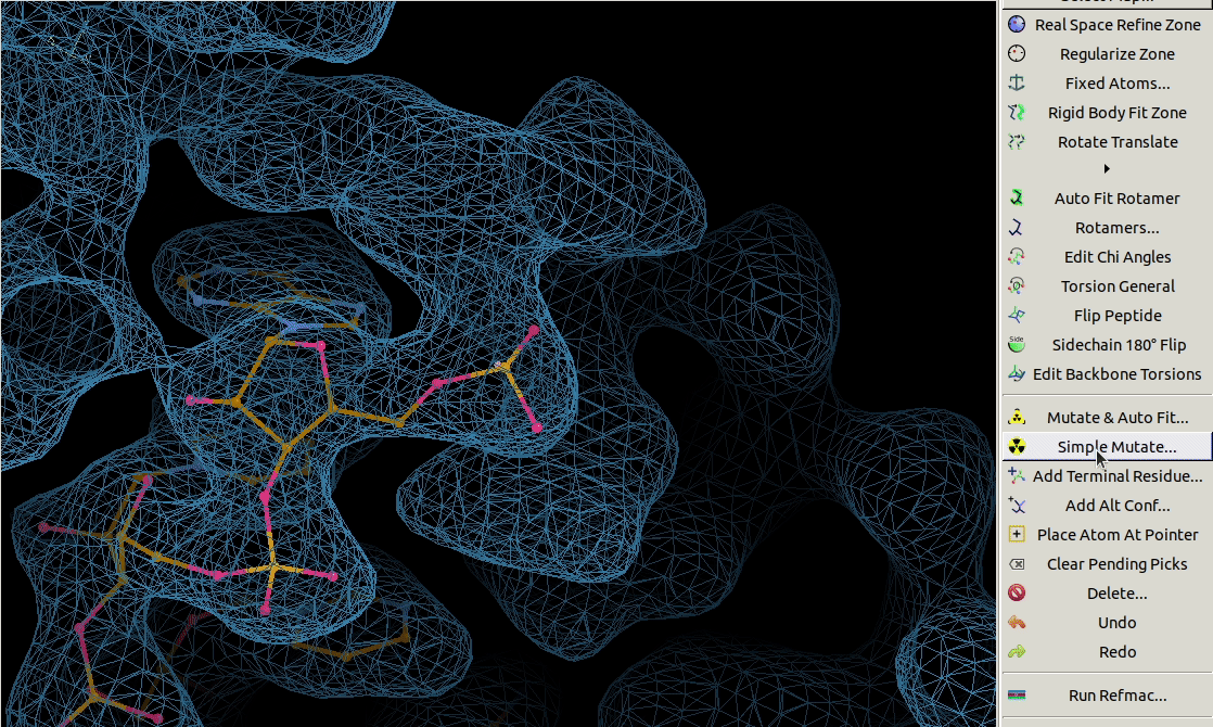
In the Other Modelling Tools toolbar,
the Base Pair tool
builds a nucleic acid opoosite the chosen one to form a bonded base pair.
In the example below we use it on a G residue
and it builds a C in roughly the right place.
3.4. Mutating Residues
Residues can be mutated individually using the Simple Mutate tool.
Afterwards they require some refinement,
which could be done using the shortcut key h,
which is similar to the triple refine t shortcut,
but it automatically accepts the refinement result.

It is also possible to mutate a range of residues using the
Mutate Residue Range tool in the Calculate menu.
You need to specify the molecule, chain ID,
a range of residues and the sequence that you want to mutate that range to.
The Autofit the mutated residues? option
may not work currently for nucliec acids
but real-space refinement can be performed afterwards.

Automatic sequence assignment and mutation can be attempted
through an automated model building program such as Nautilus within ModelCraft.
This may alter the backbone sugar-phosphate positions
but it will also try and sequence the model.
If it manages to assign a sequence it will build the corresponding bases.
For the quickest results in ModelCraft,
provide a Starting model that needs to be sequenced,
reduce the number of cycles from 25 to 1
and check the Run a quicker basic pipeline option.
Additionally, there is a new tool for identification, assignment and validation of nucleic acid sequences called doubleHelix from Grzegorz Chojnowski, which is similar in concept to the findMySequence and checkMySequence programs for protein model sequencing. This program is not yet in the CCP4 suite, but installation instructions can be found on the GitHub repository for those who are familiar with the command line.
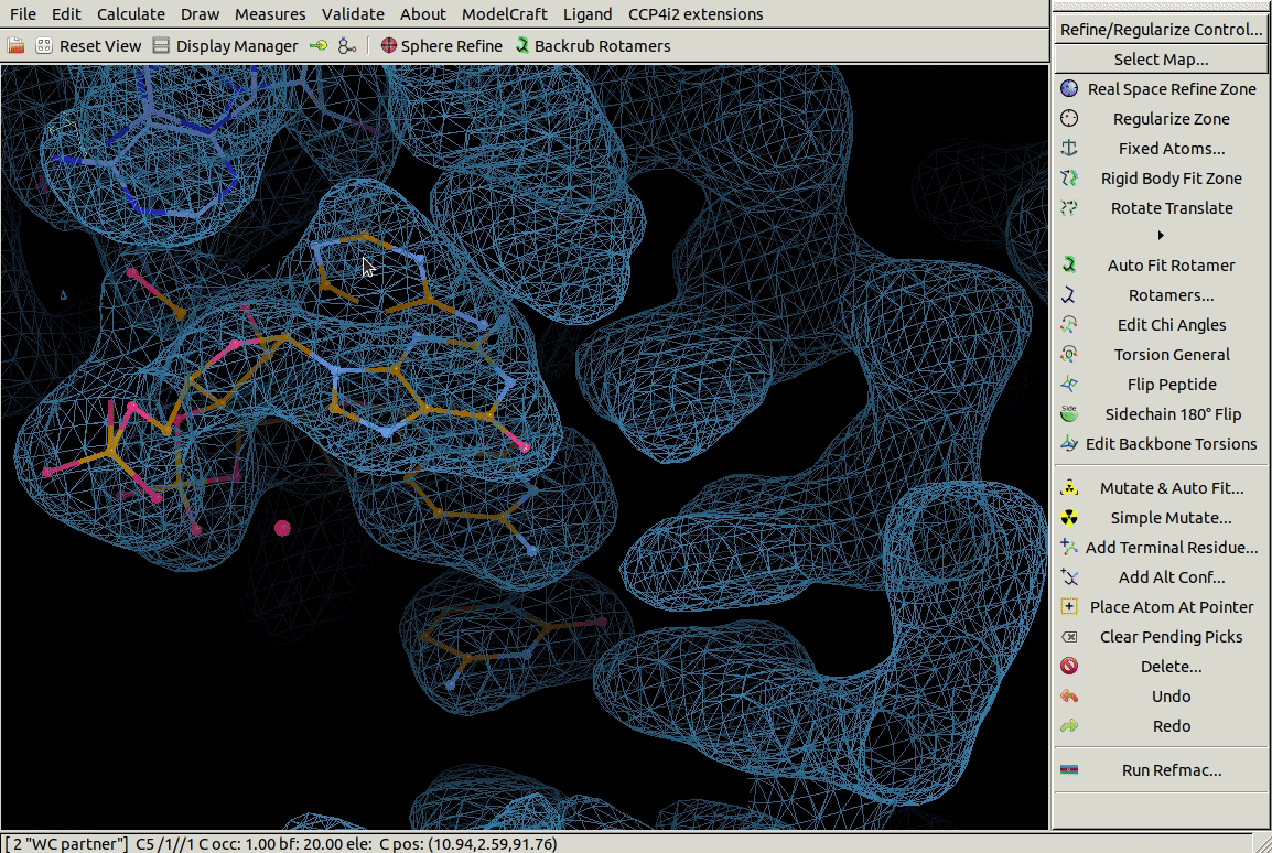
3.5. Restraints
As with standard protein residues, standard DNA and RNA residues have well-tested restraints in the CCP4 monomer library. With this high-resolution structure we are working on, the map is good enough that we can build the structure without extra restraints. However, when building into poorer maps it may help to restrain the model more. Restraints are not binary (i.e. on or off) and the weighting is important. Structures should not be under or over restrained during refinement.
Coot's real-space Refinement Weight can be changed in the
Refine/Regularize Control menu at the top of the refinement toolbar.
The default is 60.
Higher numbers use restraints less (better at higher resolution)
and lower number use restraints more (better at lower resolution).
It is worth trying the Estimate button but the estimate may not work.
If you want more restraints because your map is poor
and the estimated value is higher than 60 then overwrite it yourself.
This menu also has some general settings for real-space refinement,
e.g. to turn on Torison restraints.
There are some restraints specific to nucelic acids available in Coot.
Use the Calculate / Modules / Restraints option
to add a new Restraints menu to the top menu bar.
It has options to add RNA A form restraints, DNA B form restraints
and parallel planes restraints.
LibG (available in CCP4) and doubleHelix are programs that can be used to
automatically generate base pair and base stacking restraints.
3.6. Validation
Many of the validation tools and metrics work equally well
with both protein and nucleic acid structures.
For example the Density fit analysis graph,
which compares the average density at the atomic positions of each residue,
or the Molprobity contact analysis avalable through Probe clashes
(where pink dashes show bad overlaps).
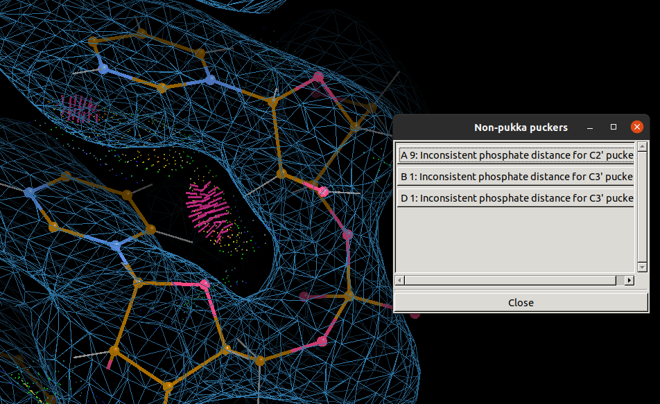
Coot also has a validation tool to analyse the ribose ring puckers
called Pukka Puckers,
which will open a window with buttons to take you to pucker outliers.
PDB-REDO validates dinucleotide conformations using the CONFAL score from DNATCO and base pair conformations using DSSR. If you create an account with PDB-REDO you can submit your own jobs to produce a re-refined version of your model with a validation report that includes these metrics.
3.7. Back to CCP4i2
After working on the model in Coot it is important to save your progress.
Use File / Save mol to CCP4i2
to choose a molecule to save to CCP4i2.
The File / Save to CCP4i2 option
will save molecule number 0 in the Display Manager to CCP4i2 (if there is one).
After this you can safely close the Coot window.
If you close the Coot window before you have saved you may lose your work.
Once the Coot window has been closed the job should be marked as finished.
At the bottom of the results page are suggestions for tasks to run next.
Clicking the REFMAC5 button opens a Refmac task
with the input parameters already filled in to refine the model saved from Coot.
After the Refmac task has finished,
clicking the COOT button at the bottom of that results page
will open a Coot task with the input parameters set
to open the model, map and difference map from Refmac.
This allows for a quicker cycle of refining, validating and rebuilding.
If you have time left, try to build as much of the 1HR2 structure as you can
starting from either the ModelCraft structure or your own model from Coot.
If you want to compare to the deposited structure, download
1hr2.cif
and use the Match model to reference structure task
to move your own model onto the same symmetry copy
before opening both models in Coot.
Paul Bond, University of York, paul.bond@york.ac.uk
CCP4i2:
L Potterton et al. Acta Cryst. D, 74, 68 (2018)
Coot:
A Casañal et al. Protein Sci., 29, 1069 (2020)