Coot Workshop
Part 1 - A Molecular Replacement Example
1. Introduction
Coot is a program for macromolecular model building, model completion and validation (Emsley et al. 2010). This workshop will give step-by-step instructions on how to use Coot to complete a molecular replacement (MR) solution. The structure we are trying to build is 5EG2, a human SET7/9 mutant in complex with S-adenosyl-l-homocysteine and a 10 residue transcription initiation factor (Fick et al. 2016). The data extend to 1.55 Å resolution and the A chain is quite small with 262 residues.
As a homology model, we have chosen 1N6A. This is an older selenomethionine derivative of human SET7/9 solved at 1.7 Å resolution (Kwon et al. 2003). The model was processed using phaser.sculptor, which trims unaligned regions using a sequence alignment and truncates side chains that differ between the model and target (pruning was not really needed in this case, but in general it is good practice). MR was done using Phaser through the CCP4i2 Basic Molecular Replacement task. This was followed by csymmatch to move the MR solution to the same origin as the deposited structure and finally refinement using REFMAC. Click the following files produced by REFMAC to download them to your computer:
- refined_model.mtz - reflection data in MTZ format
- refined_model.pdb - coordinates in PDB format
The MR solution in this example is pretty good so fixing errors directly in Coot is realistic. If the MR model was worse quality then automatic model-building software would normally be used first to complete more of the structure.
2. Starting
2.1. Starting Coot
Open a terminal and type coot.
The Coot window should appear.
For this to work, the coot executable should be in your path.
The Coot window should look something like this:
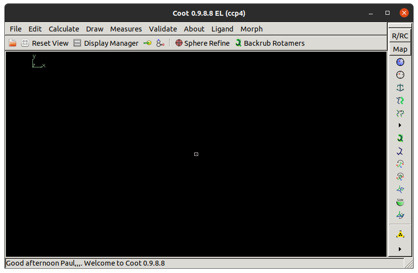
At the top of the screen is the menu bar with File, Edit, Calculate, etc. Below this is the main toolbar with a button to open the Display Manager. Buttons on the main toolbar can be customised by right clicking on the empty space. On the right is the refinement toolbar with the most widely-used model building tools. At the bottom of the window is the status bar, which is used to display messages.
2.2. Opening Files
Files that you want to open in Coot can sometimes be passed as command line arguments:
coot refined_model.pdb refined_mode.mtzFile / Open Coordinates
(you can also click the folder icon in the main toolbar).
A file browser will appear.
From this you can select a coordinate file,
as well choose how to recentre the view and the new molecule.
Select refined_model.pdb and click Open.
A window will appear asking you to fix nomenclature errors.
This is a common occurrence when opening coordinates and is usually because
there is an atom naming convention for symmetrical residues
(e.g. which way round CD1 and CD2 are in PHE)
that most programs ignore.
Click Yes to fix them.
Now we will open the 2mFo-DFc and mFo-DFc maps.
Going to File / Auto Open MTZ
is equivalent to passing the MTZ on the command line
and will open both maps if it can work out which columns to use.
We will open the maps one at a time.
Choose File / Open MTZ, mmCIF, fcf or phs
to open the file browser.
Select refined_model.mtz and click Open.
The following window should appear:
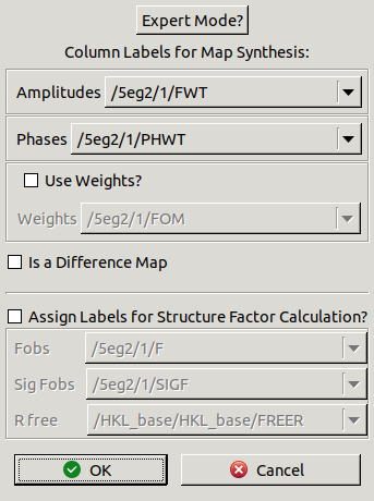
This window allows you to select
which amplitude and phase columns to use for the new map.
Defaults have been chosen for the 2mFo-DFc map.
In this case there is no need use weights
because the FWT,PHWT columns are already weighted.
If you click the Expert Mode? button
you can also choose resolution limits to truncate the data.
Click OK to open the 2mFo-DFc map.
Now we will open the mFo-DFc map.
Choose File / Open MTZ, mmCIF, fcf or phs again
and open refined_model.mtz.
Change the Amplitudes column to DELFWT
and the Phases column to PHDELWT.
The Is a Difference Map checkbox
needs to be checked (should happen automatically)
so that Coot will treat this as a difference map.
Click OK.
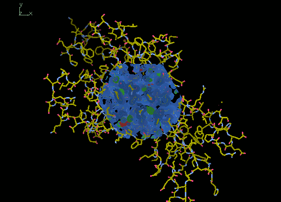
The maps should be visible as a sphere in the centre of the screen. By default, the 2mFo-DFc is coloured blue and the mFo-DFc (difference) map is coloured green for positive density (where parts of the model are missing) and red for negative density (where the model is in the wrong place).
3. Viewing
3.1. Controls
The following controls are used to change the view:
| Action | Result |
|---|---|
| Left-mouse drag | Rotate view |
| Ctrl left-mouse drag | Translate view |
| Right-mouse drag | Zoom |
| Ctrl right-mouse drag | Adjust clipping |
| Middle-mouse click | Centre on atom |
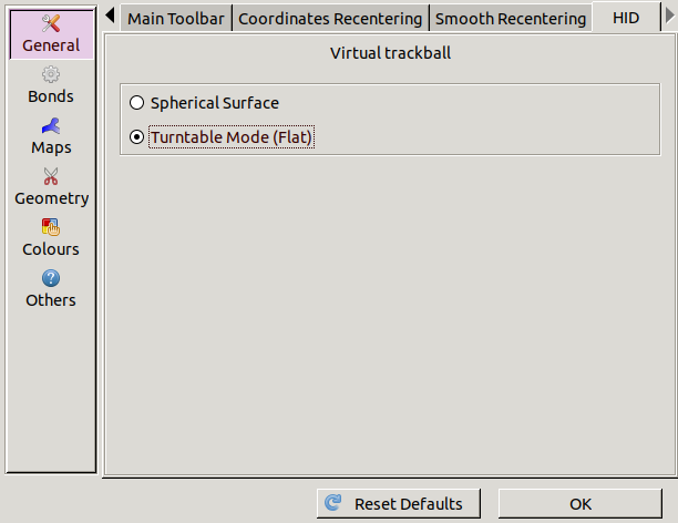
3.2. Virtual Trackball
By default, the rotation is done
using a virtual trackball with a spherical surface.
It depends not only on the direction you are dragging
but also where in the view the mouse pointer is.
If this feels strange you can try changing it
by going to Edit / Preferences,
selecting General on the left
and choosing the HID tab.
The Flat option will change the rotation
so that only the direction of dragging matters.
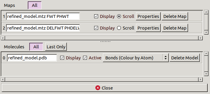
3.3. Display Manager
Open Display Manager from the main toolbar.
This shows lists of all the molecules and maps currently open.
You can toggle whether individual molecules and maps are displayed
and delete them if they are no longer needed.
You can also change map properties,
such as display style and contour levels,
and molecule representations.
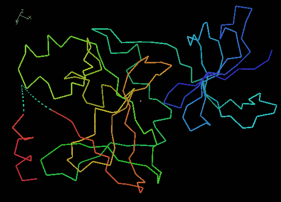
3.4. Molecule Representations
The default representation for molecules is
Bonds (Colour by Atom),
which is a good representation for model building.
However, if we want to look at larger scale features of the model
the C-alphas/Backbone representation is useful.
For now, un-display both maps
and change the molecule representation to Jones' Rainbow.
This is a variation of the C-alpha representation
where the chain is coloured
from blue at the N-terminus to red at the C-terminus.
The dotted lines at the C-terminus
show us that there are missing residues there.
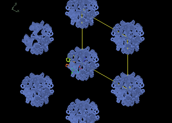
3.5. Symmetry & Packing
When checking if a molecular replacement solution is correct,
it is useful to see whether the packing of molecules
looks reasonable for a crystal.
To control the displaying of symmetry equivalents
go to Draw / Cell & Symmetry.
The following window should appear:
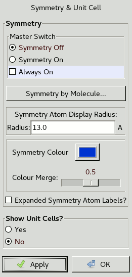
Turn the Master Switch to Symmetry On
then click the Symmetry by Molecule button
to open another window.
In the new window change the Display Options
for Molecule 0 (the only molecule)
to Display as CAs and click OK.
Increase the Symmetry Atom Display Radius
to 80 Å,
change Show Unit Cells? to Yes
and click OK.
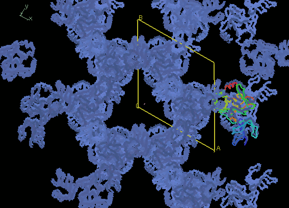
The spacegroup is P 32 2 1.
If you rotate the view to look along the C axis of the cell
you can see the threefold rotation
and long triangular channels that run through the crystal.
Also, importantly, the molecule has close contacts with its neighbours
that are necessary for crystal formation.
Below, the image on the left shows our correct MR solution.
The image on the right shows an incorrect MR solution
without proper crystal packing.
However, be sure to rotate the view to check all dimensions.
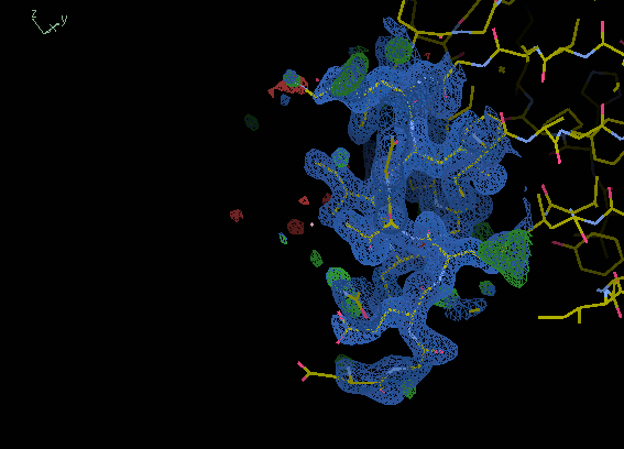
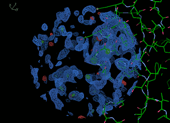
3.6. Solvent Boundaries
Another way to tell whether an MR solution is correct
is by looking at the density.
Go back to Draw / Cell & Symmetry
and change Display as CAs to Display Sphere
in the Symmetry by Molecule window.
Also reduce Symmetry Atom Display Radius
to 13 Å,
change Show Unit Cells? to No
and click OK.
In the Display Manager,
change the molecule representation to Bonds (Colour by Atom)
and display both maps.
If you move around the edge of the molecule
the density should show a clear protein/solvent boundary.
This won't be the case for a bad MR solution
as the solvent will have lots of noise.
The images below show solvent boundaries
for the correct and incorrect solutions.
3.7. Map Contouring
The maps can be contoured at different levels using the mouse scroll wheel
or + and - on the keyboard.
Density levels are specified either
as absolute values (e/Å3)
or as RMSD values.
Coot will try to pick sensible defaults on opening,
e.g. 0.41 e/Å3 (1.5 RMSD) for our 2mFo-DFc map
and 0.39 e/Å3 (2.98 RMSD) for our mFo-DFc map.
The contour level changes by steps of 0.1 RMSD.
Map properties can be edited globally at Edit / Map Parameters
and for individual maps via the Display Manager.
It is common to use RMSD when talking about map levels
but keep in mind that, as the model improves,
features in the difference map will start to disappear
so the same level RMSD will display weaker features and more noise.
3.8. Go To Atom
A useful way to move about in Coot is to use the Go To Atom window.
This can be accessed through Draw / Go To Atom,
pressing F6 on the keyboard
or clicking the ![]() icon
in the main toolbar.
icon
in the main toolbar.
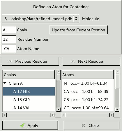
An atom can be selected using text boxes in the top left
or the lists at the bottom of the window.
Clicking Apply will move the view to the selected atom.
This window can also be used to skip through residues using the
Next Residue and Previous Residue buttons
(although it is much quicker to use
Space and ShiftSpace
on the keyboard).
Go to Glu72, which has its side chain in the wrong conformation.
The clear density for the correct side chain position
(where there is no model)
is another good indicator that the MR solution is correct.
There is also a quicker method
of going to a specific residue using the keyboard.
Press CtrlG
and a text box should appear at the bottom left of the window
(or possibly outside of the window).
Type 161 and press Enter to go to residue 161.
If the molecule has multiple chains
you can prefix the residue number by the chain label.
4. Fixing the protein
4.1. Renumber Residue Range
When preparing the molecular replacement model,
the residues were numbered so that they start from 1
at the N-terminus of the crystallised construct
instead of the N-terminus of the full length protein.
Residue 161 is actually the mutated N265A
so we need to renumber the residues to make them match up.
Go to Edit / Renumber Residues
to get the following window:
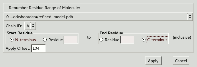
We want to renumber all residues in our chain
so change the Start Residue to N-terminus
and the End Residue to C-terminus.
Residue 161 needs to become 265
so Apply Offset should be 104.
After clicking Apply you should see the updated atom label.
4.2. Density Fit Analysis
This workshop will not go too much into validation
as it will be covered in other sessions,
but we will briefly go through density fit analysis
as it is very useful for getting a quick overview of a model.
The density fit of a residue is measured using
the average electron density level at the atom centres.
Open the analysis window by choosing
Validate / Density fit analysis
and picking the molecule.
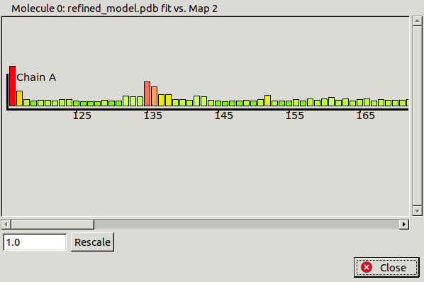
A window like the one above should appear. It shows a graph of residue number against density fit for each chain. Residues with good density fit values are small and green, and bad density fit values are large and red. If all residues are showing as green or red then the scale should be adjusted using the controls in the bottom left. In this case we can see some residues with poor fit to density, mainly at the N and C termini. Click on the bar for His116 at the N-terminus to move the view there.
4.3. Deleting
Because the density for His116 is not very good
we may want to delete this residue.
The delete button can be found at the bottom of the refinement toolbar.
If you are unsure which buttons correspond to which functions
you can add text via Edit / Preferences.
In the Refinement Toolbar tab
of the General section,
change the Toolbar Style
from Icons only to Icons and Text.
Click the Delete button and the following window should appear:
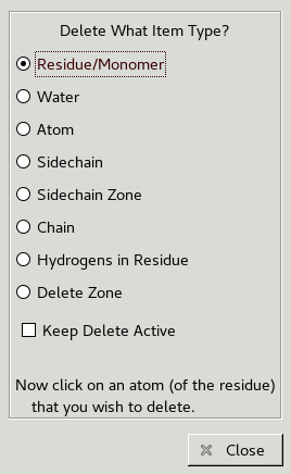
Now click on one of the atoms in His116 to delete the residue.
Individual atoms (or side chains) can be deleted in the same way
by selecting this option in the window before clicking.
You can check Keep Delete Active to keep the delete window open
so that multiple residues can be deleted.
If the residues are sequential
it might be easier to use Delete Zone.
In this case you need to click twice:
once on the first residue to be deleted and once on the last.
4.4. Mutating
All of the residues in this structure are the correct type
so do not need mutating.
However, quite a few of the residues do not have complete side chains
and the mutate function will also work to rebuild them.
Go to Met139 and see that the side chain is not complete.
There is even a loose atom claiming to be the CE atom.
It must have been left there during model preparation
and this is the position it ended up in after refinement.
There is clear difference density
where the side chain is supposed to go.
Click on the Simple Mutate button in the refinement toolbar
then click on an atom of Met139.
A list of residue types should appear.
Click on MET and the side chain will be completed
(although not in the right conformation).
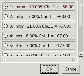
4.5. Rotamers
Now we need to move the side chain into the correct conformation.
Click the Rotamers button in the refinement toolbar
and then click one of the atoms in Met139.
A list of rotamers for that residue type appears.
A rotamer is simply a commonly observed side chain conformation
and this list is ordered from most to least common.
Use . and , on the keyboard
to cycle through the rotamers when the main Coot window is selected.
This can be done while adjusting the view in the main window.
Each rotamer has a name that roughly describes the chi angles:
p for 60°, m for -60°, t for 180°,
and a number for the final angle of sp2 side chains.
The closest rotamer for Met139 is mmt.
Select this and click OK.
Press x to perform real space refinement on this rotamer,
which moves it into the density
(as long as the residue is at the centre of the view).
If this doesn't work you first need to click
Edit / Settings / Install Template Keybindings.
There is also an Auto Fit Rotamer button in the refinement toolbar
that will try to pick the closest rotamer and then refine it automatically.
Click this and then an atom of Met139 to try it out.
The keyboard shortcut for this is j,
which auto-fits the rotamer at the centre of the screen.
There is another useful button on the refinement toolbar
that automates everything we did in the last two sections.
Go to Met164, click Mutate & Auto Fit,
then click an atom from the residue and select MET from the list.
4.6. Real Space Refinement
The aim of real space refinement is to move the atoms
so that two scores are improved:
one is how well the atoms fit the density
and the other is how close bond lengths, angles, etc are to ideal values.
Parts of the second term are known as restraints.
At high resolution you can see individual atom positions
so the density score is more important than the restraints score.
At low resolution the density is not as detailed
so the restraints score becomes more important.
To adjust the weighting between the two scores,
select Refine/Regularize Control
at the top of the refinement toolbar.
You can change which restraints to use as well
as the weight between the density and restraints terms.
The default is 60.
Higher numbers will use the restraints less.
Click the Estimate button,
which will try to choose a sensible weight for the current map.
If you have multiple maps open,
the map that you are refining into can be changed
with the Select Map button underneath.
Go to Thr175. The red density at CG2 and strong green density opposite
tell us that the side chain needs rotating.
Instead of auto-fitting the rotamer we will attempt to refine it manually.
Click the Real Space Refine Zone button
on the refinement toolbar then click on Thr175 twice.
You need to click twice because it expects a zone,
i.e. you need to click the first and last residue
in the range you want to refine.
Some refinement traffic lights will appear:
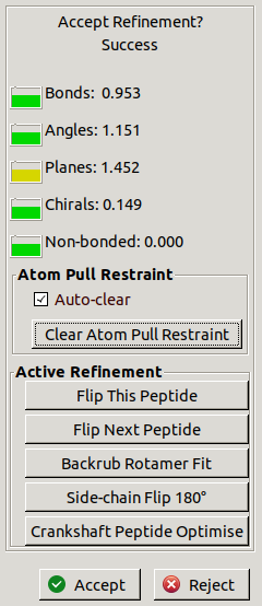
The numbers show
how many standard deviations the restraints are from their ideal values.
There is also a simple traffic light system
showing (from good to bad) green, yellow, orange and red.
The fit to density can be assessed by eye.
An initial minimisation has been done
and the result is shown as a white copy of the atoms.
They haven't moved much as the conformation is at a local minimum.
Click the OG1 atom, drag it to the green density and let go.
In older versions of Coot (pre-0.9) you had to over-drag,
i.e. drag the atom past where you wanted it to end up,
but this is no longer the case.
Once the residue is rotated into the right place click Accept.
The shortcut we used earlier for refinement was x,
which refines the residue at the centre of the view
and automatically accepts the initial minimisation.
If you want to drag the atoms or look at the refinement traffic lights
you can use the r key instead.
It is usually preferable to include the residues either side
when refining so the backbone geometry does not become distorted.
This is known as triple refine or neighbours refine.
The shortcut for this is t (without auto-accept)
or h (with auto-accept).
A powerful combination of shortcuts is hjh,
which can correct most side chain errors.
It does neighbours refine to minimise the backbone geometry,
auto-fits the rotamer
(which should be easier with the updated backbone positions)
and finally another neighbours refine
to remove any backbone distortions introduced during the rotamer fitting.
Press space to go to Glu176
and then hjh to fix the rotamer.
4.7. Alternate conformations
Press space to go to Glu177.
There is clear positive difference density
suggesting the side chain should be in another conformation.
There is also some negative difference density at the current position
but auto-fitting puts the rotamer back in the same place.
In this case the side chain could exist in two conformations in the crystal
and the negative difference density
is because we only have one at 100% occupancy.
Press the Add Alt Conf button on the refinement toolbar.
The following window should appear:
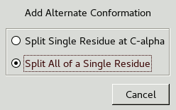
This lets you choose whether to split the whole residue or just the atoms from C-alpha onwards. Splitting the whole residue will allow for any slight changes in backbone conformation. Now click on an atom in Glu177 and another window will appear:
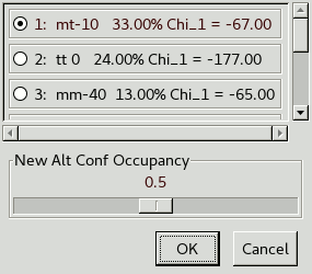
This lets you select an initial rotamer for the new conformation
as well as what occupancy you want it to have.
In this case we will leave the occupancy at 50%.
After doing global refinement with REFMAC
you may notice difference density
that suggests the occupancy should be different
(REFMAC is also able to refine the occupancy).
Look through the rotamers with . and ,,
select the one you think is closest and click OK.
Perform a neighbours refine (h or t)
to clean up the positions of both conformations.
4.8. Adding Terminal Residues
Between Tyr337 and Pro350 there is a missing loop
with the sequence DHSPPGKSGPEA.
However, we have enough density to build some of the residues.
Go to Tyr337,
click Add Terminal Residue on the refinement toolbar
and click on an atom of Tyr337.
This will build an alanine as the next residue.
Press h to refine it, mutate it to aspartic acid,
then fit the rotamer and refine again.
Go to Pro350 and do the same for the other end of the loop.
The backbone is quite clear for Ala349 and Glu348.
There is some density for Pro347
but you might want to wait until doing more refinement
to get an improved map.
4.9. Peptide bonds
There is a problem with the peptide bond between Glu279 and Pro280.
You will see there is negative difference density at the carbonyl oxygen
but positive difference density opposite.
This is a sign that the peptide needs to be flipped.
Usually, this can be fixed by clicking on
the Flip Peptide button on the refinement toolbar
and clicking the peptide.
The shortcut q flips the peptide at the centre of the view
and hqh is another useful key combination.
However, in this case there is an extra complication.
Flipping the peptide will flip both the carbonyl and the nitrogen
and still form a trans-peptide.
If you try to refine this you will end up with a twisted peptide
where the omega angle is > 30° and < 150°.
This is indicated by a yellow shaded area.
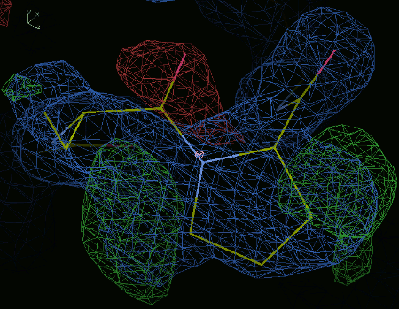
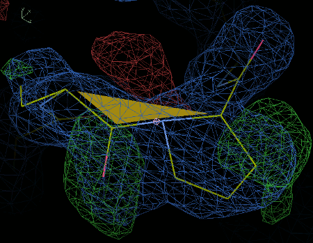
This example should be a cis-peptide instead.
Click the Edit Backbone Torsions button
on the refinement toolbar and then click an atom of the peptide.
This allows you to rotate either the whole peptide bond
or just the carbonyl using sliders.
A Ramachandran plot for the residues either side gets updated as you rotate.
One of the residues starts in the white disallowed region of the plot,
which also suggests something could be wrong.
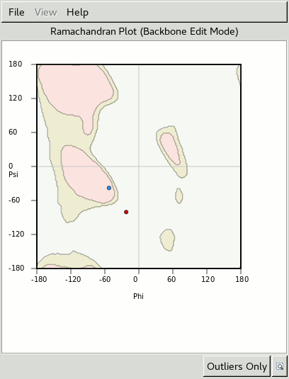
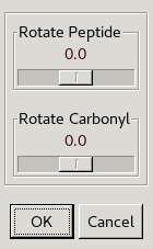
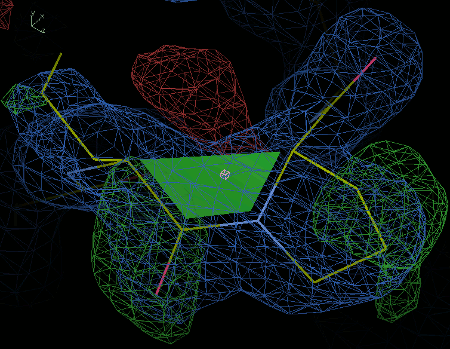
Use the slider to rotate the carbonyl into the middle of the green density
and click okay.
You should hopefully see a green shaded area to indicate that
it is a now a cis-peptide bond as the omega angle is less than 30°.
This is important because
if there is a yellow shaded area for a twisted peptide
then trans-peptide restraints will be used.
These can be temporarily turned off
from Refine/Regularize Control
if you are struggling to force the backbone into the correct conformation,
but in general they should be kept on
to avoid building incorrect cis-peptides.
Cis-peptides are only common for X-Pro bonds.
If the second residue is something other than proline
then a red shaded area will be shown to indicate a possible error.
The figure below shows the correct conformation.
5. Adding ligands
5.1. Unmodelled blobs
The protein has two ligands that needs to be modelled:
a 10-residue peptide and S-adenosyl-l-homocysteine.
There is a useful tool that finds ligands and solvent molecules
by looking for blobs of density that have no model
and are too big to be water molecules.
Go to Validate / Unmodelled blobs
to get the following window:
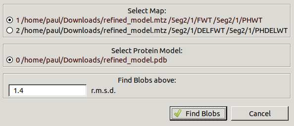
Leave the defaults and click Find Blobs
to search the 2mFo-DFc map for blobs above 1.4 RMSD.
A list of unexplained blobs should appear.
Click through the blobs to find the density for the peptide
(it should look like the density in the image in the next section).
5.2. Building a short peptide
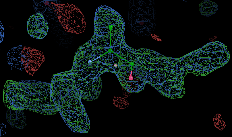
The clearest density is probably in the middle of the blob
where there is a long lysine derivative
with some side chain density between Tyr245, Tyr305 and Tyr335.
We will start by placing an alanine at this position.
First, move the view centre to where you want the residue to be,
then go to Calculate / Modelling / Monomer from Dictionary.
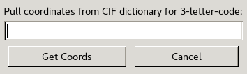
This window is used to get coordinates for a ligand
that already has a restraints dictionary in the CCP4 monomer library.
Type ALA in the box and click Get Coords
to place an alanine ligand at the centre of the view.
The new alanine will have more atoms than we need.
Delete the hydrogen atoms and the OXT atom (not O)
using Delete in the refinement toolbar.
Then use interactive real space refinement
to drag it into the correct position.
This residue can now be treated the same as any other peptide.
Use Add Terminal Residue to add
one extra residue to the C-terminus and two to the N-terminus.
Past this point
the positions are not very well supported by the density yet.
Make sure to refine each residue into position after it is added.
This method for building a polyalanine chain
is good for a short peptide ligand,
but for longer chains the baton building mode should be used
(which is covered in part 2 of the workshop).
5.3. Merge molecules
As you can see if you open the Display Manager,
the peptide ligand is currently in a separate molecule
when it should be the B chain of the same molecule.
Go to Edit / Merge Molecules to get the following window:
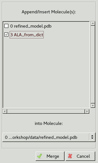
The molecules checked at the top of the window will be copied
into the molecule chosen at the bottom.
In this case we want to copy the alanine ligand into the main molecule.
It will automatically be labelled as chain B.
The ALA_from_dict molecule can now be deleted
using the Display Manager.
5.4. Mutate residue range
The sequence for the peptide is SKSKDRKYTL (Ser186 to Leu195).
The four residues we have built so far
are KSKD (Lys187 to Asp190).
First use Edit / Renumber Residues to fix the numbering
then click Calculate / Mutate Residue Range
to open the following window:
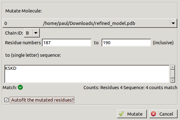
Make sure the inputs match those in the picture above. The auto-fitting rotamers is optional as you will probably find you need to follow this up by more real space refinement and manual adjustment of the side chains. The density for Lys187 is not very strong so it may be better to delete this side chain.
5.5. Modified residues
Go to the B:Lys189 residue that we have just built.
This should actually be N-methyl-lysine (MLZ).
To mutate it make sure the residue is at the centre of the view
and click Edit / Replace Residue.
A window will appear where you can type the 3-letter code.
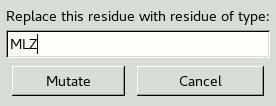
Type MLZ and click Mutate.
The LYS should be replaced with an MLZ residue
in roughly the same place and with the same numbering.
It will need refining (e.g. shortcut h)
to move it back into place.
5.6. Adding a known ligand
This section will deal with placing a ligand
that is already in the monomer library.
Run Validate / Unmodelled blobs again with the default options
and select the remaining blob for S-adenosyl-l-homocysteine.
Go to File / Search Monomer Library,
which allows you to search for monomers by name.
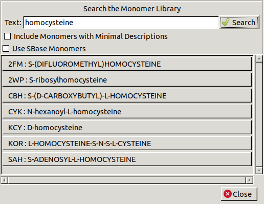
Type homocysteine in the textbox and click Search.
Then select SAH from the list
to place the residue at the centre of the view.
We will first attempt to fit the ligand into the density manually.
Select Rotate Translate in the refinement toolbar
and click on SAH twice.
This brings up a window with sliders to adjust
rotation and translation about the X, Y and Z axis.
The axes are relative to the view and not the coordinate axes:
X is left to right, Y is top to bottom and Z is perpendicular to the screen.
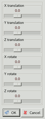
Use the sliders to get the orientation of the ligand roughly correct,
then use real space refinement to try and drag the atoms into place.
If you are struggling to get the molecule into place
try Ligand / Jiggle-Fit Ligand,
which automatically tries different positions and orientations
with rigid-body and real-space refinement.
Now we will look at the more automated way of fitting ligands.
First, delete the manually fitted SAH_from_dict molecule.
Go to File / Get Monomer,
which can be used instead of Search Monomer Library
if you already know the three letter code.
Type SAH and click OK.
As we know which blob the ligand should be in,
centre the view there and then click Ligand / Find Ligands.
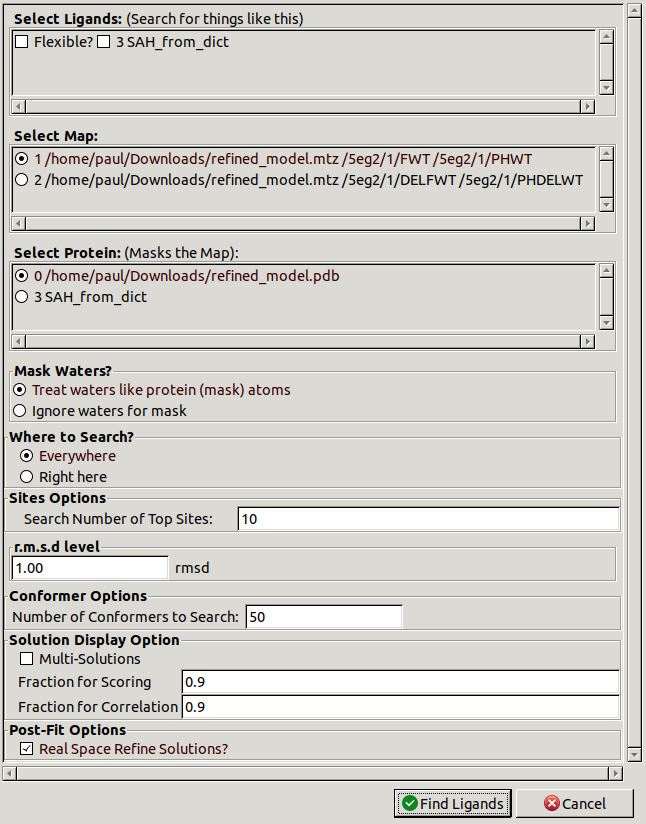
In the Select Ligands section,
choose the newly placed SAH_from_dict ligand.
Change Where to Search? to Right here.
If you did not know where the ligand should go then
you could use Everywhere.
You could also increase Number of Conformers to Search.
This will take longer but have more chance of fitting the ligand correctly.
Ligands with more rotatable bonds are likely to need higher numbers.
Click Find Ligands to start the search.
A new molecule will be made for the fitted ligand.
If the correct conformation is not found then delete this new molecule
and try running Find Ligands again with more conformers
and possibly changing the center of the view within the blob.
Otherwise, use Merge Molecules to merge it into the main molecule
then delete the other molecules.
The fit may not be exact and may still need some interactive refinement.
You should also delete the hydrogen atoms of the ligand
as these are not usually included in a model
except for very high resolution cases where they are observed.
6. Adding waters
6.1. Automatically
The structure we are working on is quite high resolution
so there are lots of peaks for ordered water molecules around the protein.
Fewer waters are seen as you move to lower resolution
and they stop being visible somewhere around 2.5 to 3.0 Å.
Go to Calculate / Other Modelling Tools
to open another toolbar
and select Find Waters.
Leave the default settings and click Find Waters.
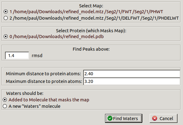
A new chain will be made in the molecule to contain the new waters.
The waters should be checked by eye.
Use Go To Atom to move to the first water in this chain.
Then it is useful to see what hydrogen bonds the water is making.
Choose Measures / Environment Distances,
check Show Residue Environment? and click OK.
Then press space to move through the water molecules
and examine them one at a time.
To make the view always jump from one atom to the next
instead of sliding,
turn off Smooth Recentering
in the General section of Edit / Preferences.
There is no need to check all the waters during the workshop
but you should when working on your own structure.
6.2. Individually
Automatic water finding will miss some waters that can be built manually.
In order to find peaks that might be water molecules,
go to Validate / Difference Map Peaks.
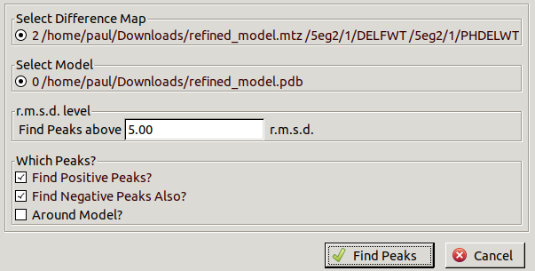
Leave the default 5.00 r.m.s.d.
but uncheck Find Negative Peaks Also?
as peaks for missing waters will be positive.
Use . and , to move up and down the list
when the main Coot window is selected.
The biggest difference map peaks
are for the missing sulfur atoms in the methionine residues.
Keep looking until you find a peak for a water molecule
that hasn't been added automatically.
Most of the peaks will have been modelled already
so it would be better to do this after another round of refinement.
Once you have found one,
click Place Atom At Pointer then OK
to add a water molecule.
You can also use the shortcut w on the keyboard.
Press x to refine the water position.
Remember to save your improved model using
File / Save Coordinates.
Part 2 - Building From Scratch
Paul Bond, University of York, paul.bond@york.ac.uk